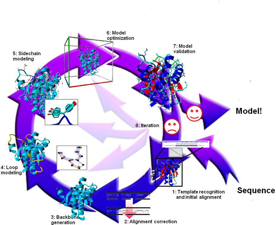
Figure 25. The eight steps of homology modelling.
|
After the homology modelling practical you will: Understand the basic concepts of homology modelling; Understand the relation between homology modelling and the other parts of the course (validation; alignment; docking; force fields; MD); Be able (in principle and when the model is not overly complicated) to build your own model, and to look at it with YASARA. |
The remainder of this section is produced from the homology modelling article; and contains more information than you will need. The questions in the practical and in the example exams indicate which aspects of this article are considered important concepts. It is nearly certain that the exam will contain a question about the Force Fields involved in the Homology Modelling process. These Force Fields will be discussed at a later stage during this course.
Homology modelling is usually described as a multi-step process in which the number of steps typically varies wildly. Here we use an eight step plan. Over the years each of these eight steps has undergone extensive scrutiny and has been the topic of much research. Consequently, models built today with a fully automatic web server are considerably more accurate than the first model-approach four decades ago by Browne et al. using wire and plastic models of bonds and atoms (Browne et al. 1969).
|
|
Figure 25. The eight steps of homology modelling. |
The first step involves finding a suitable, homologous protein of which the structure can be used as modelling template, and generating the initial alignment between that template and the model sequence. In step 2 this alignment is refined using, for example, knowledge obtained from the template structure. In step 3 the backbone is generated and deletions are performed so that, temporarily forgetting insertions, the backbone of the template looks like that of the model as much as possible. In step 4 gaps in the model are closed, and optionally loops are ab initio constructed. In step 5, the side chains are added using rotamer libraries to find the best rotamer for that local backbone conformation. Step 6 consists of a molecular dynamics simulation on the complete model in order to remove (the majority of) the introduced errors. In step 7 the model is checked for remaining errors using validation software. Depending on the outcome of the validation step we either approve the model or iterate the modelling process (step 8), starting from step 1-6.
Question 4: About a year from now, most of you will be starting the first master internship. Try to come up with project titles for 5 putative master internships that will include homology modelling. These 5 internships should take place in 5 (very) different departments. Explain how homology modelling will be needed in that project. (Feel free to skip this question...
Answer
Question 5: What does it mean if two proteins are homologs of each other?
Answer
Question 6: Upon homology modelling we speak of the template and the model. What are those?
Answer
Question 7: The word rotamer has two similar, but different, meanings. If we use the meaning 'all possible conformations of the side chain' why do we then observe three rotamers for residues such as serine, cysteine, and valine (look them up on the orange sheet)?
Answer
Traditionally, the modelling template is found by performing a BLAST (Altschul et al. 1990) search against the Protein Data Bank [PDB] (Berman et al. 2003). This approach is often successful when the query is highly identical to structures in the database. In contrast, templates that are close to the possible homology modelling threshold are harder to find or may even remain undetected (Sander and Schneider 1991). The development of PSI-BLAST (Altschul et al. 1997) and fold-recognition methods (e.g. Jones 1999) improved the detection of these difficult-to-find templates because these methods use a profile instead of a single sequence to search the database. Furthermore, the growing number of structures collected in the PDB makes it easier every year to find a homologous one.
In the box below you find a sequence. This could, for example, be the sequence of a protein for which we need a model.
>My_beautiful_sequence AAATGSGTTLKGATVPLNISYEGGKYVLRDLSKPTGTQIITYDLQNRQSRLPGTLVSSTTKTFTSSSQRAAVDAHYNLG KVYDYFYSNFKRNSYDNKGSKIVSSVHYGTQYNNAAWTGDQMIYGDGDGSFFSPLSGSLDVTAHEMTHGVTQETANLIY ENQPGALNESFSDVFGYFNDTEDWDIGEDITVSQPALRSLSNPTKYNQPDNYANYRNLPNTDEGDYGGVHTNSGIPNKA AYNTITKLGVSKSQQIYYRALTTYLTPSSTFKDAKAALIQSARDLYGSTDAAKVEAAWNAVGL |
Question 8: Take 'My beautiful sequence' from the box above, and use the software BLAST to find a protein structure in the PDB that can be used as a homology modelling template. You find BLAST as part of the MRS suite that you find under Pointers.
This question might be a bit over-complicated, especially since we aren't
very interested in how BLAST works, and which buttons to push, etc. Therefore,
I added some pictures as supplemental material that show you step-by-step
what to do.
At the end, look up what is the percentage identity between 'My beautiful
(model) sequence' and the best template with known structure in the PDB.
Feel free to cheat a bit and save the time of actually doing all thse things
because the example given under ′Supplemental material′ actually
used My_beautiful_sequence... :-)
Supplemental material
Finding the best possible template is not limited to searching the PDB with (PSI-)BLAST. There may be several candidate templates with similar sequence identities to the query. In that case, the optimal template must be selected based on other criteria. The X-ray resolution is, although frequently used as such, only a limited measure of structure quality because it says something about the experimental data, not about the quality of the structure model. I.e. with 1.8 Ångström data one can typically make a better structure model than with 2.2 Ångström data, but whether or not this better structure model is actually made, depends on the crystallographer and the software (s)he uses.
The Supplemental material listed here can for now be skipped, but after the validation day you are supposed to be able to at least read and understand these sections.
Supplemental material
|
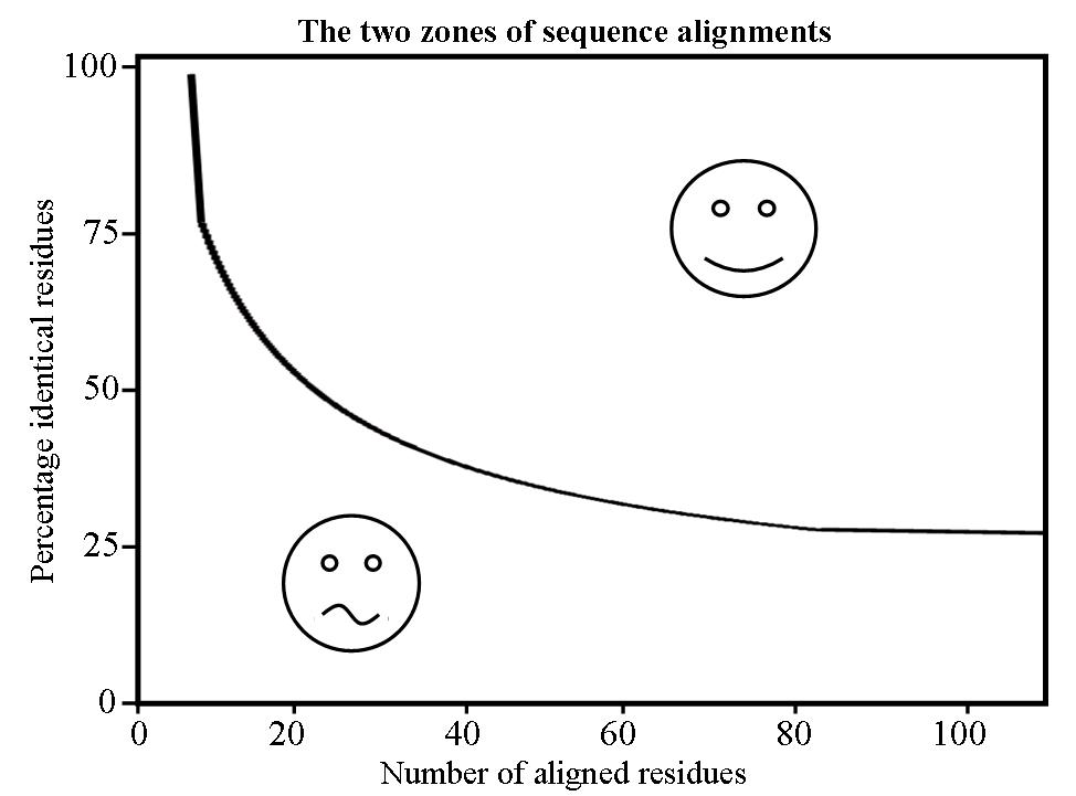
The Sander and Schneider homology modelling threshold curve. |
Question 9:
Answer
Feel free to not yet understand things written in this section. Alignment will be explained in the sequence analysis seminar.
Having identified one or more possible modelling templates using the initial screen described above, more sophisticated methods are needed to arrive at a better alignment. Molecular class-specific information systems (MCSISs) can be a great asset in the homology modelling process. MCSISs contain a large number of heterogeneous data on one particular class of proteins. The GPCRDB at www.gpcr.org/7tm/ (Horn et al. 2003) is a good example of such a system. It contains sequences, structures, mutation data, ligand binding data, and much more. All of this information is used (directly or in an indirect way) for creating sequence profiles for GPCR (sub)families. Profile-based alignments (Oliveira et al. 1993) are used to generate alignments that are of a significantly higher quality than alignments generated by automatic methods based solely on sequence data. Currently, MCSISs are available for only a small number of protein families and therefore in most cases other sequence alignment tools are needed.
Many programs are available to align a number of related sequences, for example CLUSTALW (Thompson et al. 1994). The resulting multiple sequence alignment implicitly contains a lot of additional information. For example, if at a certain position only exchanges between hydrophobic residues are observed, it is highly likely that this residue is buried. Multiple sequence alignments are also useful to place deletions or insertions in areas where the sequences are strongly divergent. To consider this knowledge during the alignment, one uses the multiple sequence alignment to derive position specific scoring matrices, also called "profiles" (e.g. Taylor 1986, Dodge et al. 1998). In recent years, new programs like MUSCLE and T-Coffee have been developed that use these profiles to generate and refine the multiple sequence alignments (Edgar 2004, Notredame et al. 2000).
When building a homology model, we are in the fortunate situation of having an almost perfect profile: the known structure of the template. We simply know that a certain alanine sits in the protein core and must therefore not be aligned with a glutamate. Alignment techniques like SSALN make use of this structural knowledge found in the template (Qiu and Elber 2006).
Question 10: In the list of exercise files you find the files 1PPT.pdb and 1PP2.pdb. Open two YASARA windows and look at 1PPT with the one YASARA, and at 1PP2 with the other.
Now write in the sequence box underneath each residue in the 1PPT sequence the residue type of the residue in 1PP2 that sits at the equivalent position. If there is is a residue in 1PPT but there is no residue at the corrsponding location in 1PP2, simply write a dash. This exercise is best done if you work in teams of two people...
1PPT: GPSQPTYPGDDAPVEDLIRFYDNLQQYLNVVTRHRY 1PP2 |
Answer
Well, that was your first alignment. In a sequence alignment we want to write underneath each other those residues that sit at equivalent ( homologous) positions in the structures. You could have achieved the same result using a sequence alignment program like CLUSTAL. In the same MRS that you used before you find a version of CLUSTAL. In the supplemental material you see how you can use CLUSTAL to get an alignment between the two sequences.
Supplemental material
Question 11: Are the two alignments the same? I.e., is the alignment you made by comparing the structures the same as the alignment CLUSTAL made by comparing just the sequences?
Answer
Among the exercise files you find the structure CRAS.pdb and the model CRAM.pdb. You also find their two sequences, call CRAS.pir and CRAM.pir, respectively. Align the two sequences with CLUSTAL and store the result 'somewhere'. You see that CRAM is missing two residues. And we know that if there are alignment problems, these tend to be near insertions/deletions.
So, lets look at the two structures, and see what we think about this CLUSTAL alignment. To make this a bit easy, you should load the file CRASCRAM.sce that is also present among the exercise files. This scene file holds the two structures, CRAS and CRAM, nicely superposed.
Question 12: Make a structure alignment (like you did earlier for 1PPT and 1PP2) for CRAS and CRAM. Don't do the whole forty-something residues. CLUSTAL can do that for you. Just look around the deletion, because if anything went wrong in the CLUSTAL alignment, then it went wrong just there.
Now write the structure alignment (or at least the relevant part) under the sequence alignment. You see they are different. What is different? What happened in evolution that caused this difference?
Answer
The validation part of this section will become clear after the validation seminar (and practical). Feel free to not yet understand everything in this section.
Aligned residues occupy similar positions in template and model. Coordinates can thus simply be copied over to create the initial model backbone. In practice, there are many ways to improve this crude recipe. First, the template sometimes is present more than once in the PDB (e.g. a bundle of NMR structures, multiple copies in the crystal, or solved multiple times under different conditions). Here, one can use structure validation tools (Hooft et al. 1996a, Laskowski et al. 1993), like the PDBREPORT databank at www.cmbi.umcn.nl/gv/pdbreport/ to pick the best one, correcting errors where possible. Second, one can combine multiple templates, because residues missing in one template can sometimes be found in the other, or because the alignment covers more than one template, which is common for multi-domain targets. The well known SwissModel server (http://swissmodel.expasy.org/ Arnold et al. 2006) selects fragments from different PDB files that locally are most similar to the corresponding model fragment. The Zhang (http://zhang.bioinformatics.ku.edu/I-TASSER/ Pandit et al. 2006) and Robetta (http://robetta.bakerlab.org/ Chivian et al. 2003) modelling servers have successfully extended on this concept and are today among the best homology modelling servers available on-line. Some methods do not even create a single backbone at all, instead they use the alignment to derive restraints (hydrogen bonds, backbone torsion angles, etc.), and only later build the model, while trying to satisfy the restraints (Modeller, Sali and Blundell 1993).
Lets take an example, and see how much error we make by all these assumptions about the backbone. Lets take a look at two molecules: 1CRN and 1ED0. They are homologous as you can see from their sequence alignment. But you can see it even better from their superposed structures:
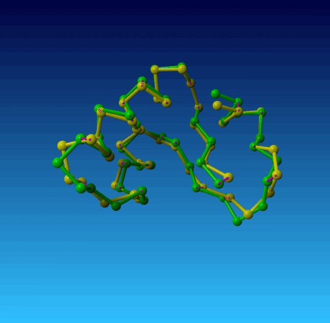
|
1CRN in green and 1ED0 in yellow. Only the Cα atoms are shown. The structure differences (for Cαs) are indicated with small purple lines ( unless the difference is too big). This scene is available as exercise file 1CRN1ED0.sce. |
Question 13: The sequence alignment of 1CRN and 1ED0 is:
1CRN: TTCCPSIVARSNFNVCRLPGTPEAICATYTGCIIIPGATCPGDYAN 1ED0: KSCCPNTTGRNIYNACRLTGAPRPTCAKLSGCKIISGSTCPSDYPK |
Study the differences. Indicate in the alignment the four areas where the backbone
differences are largest. Where do you see the most striking differences?
Now go back to what you know about the amino acids. Which amino acids behave different from
all others in terms of backbone conformation? And which residues have been mutated
between 1CRN and 1ED0 in the two loops that differ most between them?
Any insertion or deletion in the alignment implies a structural change of the backbone, and can thus not be modelled in the previous step. Since these changes usually take place outside regular secondary structure elements, their prediction is referred to as loop modelling. There are two major approaches to the problem: first knowledge-based methods (Michalsky et al. 2003), which search the PDB for known loops with high sequence similarity to the target and endpoints that match the anchor residues between which the loop has to be inserted. And second energy-based methods, which sample random loop conformations while minimizing an energy function (Xiang and Honig 2002). Since loops never fit the anchor points exactly, they have to be closed, using for example an algorithm borrowed from robotics (Canutescu et al. 2003a). In practice, a combination of both methods is common.
The most successful approaches to side chain prediction are knowledge-based. They use libraries of common side chain rotamers extracted from high resolution X-ray structures (Dunbrack and Karplus 1993, Chinea et al. 1995, Lovell et al. 2000). An essential feature of these libraries is backbone-dependence, hence they store the distribution of the side chain dihedral angles (χ1, χ2, etc.) as a function of the backbone dihedrals φ and ψ. This does not only increase the accuracy, but also helps to shrink the search space (i.e. the possible combinations of interacting side chain rotamers) to a size that can be handled, for example using dead-end elimination (Canutescu et al. 2003b). The prediction accuracy is usually highest for residues in the hydrophobic core, where more than 90% of all predicted χ1-angles fall within 20o from the experimental values, but significantly lower for residues on the surface where the percentage drops to 70%, and further down to 50% for the combined χ1/χ2 accuracy (Canutescu et al. 2003b). This is mainly caused by the electrostatic and hydrogen bonding interactions, which are partly solvent mediated and much more difficult to get right than the simple repulsive Van der Waals interactions in the core, but also partly due to the fact that flexible side chains on the surface tend to adopt multiple conformations, which are additionally influenced by crystal contacts, so there simply may not be a single correct conformation at all. Nevertheless, the surface residues are among the most important ones to get right; they mediate all the interactions, and applications like drug design or protein docking thus critically depend on them.
Question 14: YASARA has the option 'Rotamers of' in the 'Analyze' menu. Try to describe what this option does. (Actually, the YASARA installed by CNCZ doesn't have this option... When you need to calculate rotamers, check the FILES list because for each rotamer calculation a YASARA-scene has been stored with that rotamer search done for you).
Answer
Question 15: Start YASARA and read CRAS.pdb. Run the 'Rotamers of' option on Val-15. Discuss what you see.
Answer
Question 16: Run the 'Rotamers of' option on Phe-13. Discuss what you see.
Answer
Question 17: If we had to model a phenylalanine at position 13 in CRAS, we would have to choose from among two likely rotamers. What would you (or what does modelling software do) do to make a decision?
Answer
Once all these steps are completed, one obtains the initial homology model, which hopefully looks broadly similar to the (usually unknown) target structure. The little details however, like the precise backbone conformation, hydrogen bonding networks or certain side-chain rotamers, are often wrong. While this deficiency keeps scientists working on experimental structure determination busy, predictors strive to bridge the gap between model and target (the 'last mile of the protein folding problem') using various optimization and refinement techniques, the most prominent ones being molecular dynamics (Krieger et al. 2004) and Monte Carlo simulations (Misura 2006). For a given model, there are unfortunately many more paths leading away from the target than towards it, and combined with the limited accuracy of empirical force fields, this makes it trivial to reduce the model accuracy during the refinement. Consequently, the best optimization was often no optimization. We did well in the early CASP homology modelling competitions simply by not performing MD simulations on the models (except for 25 energy minimization steps with CNS (Brünger et al. 1998) to introduce the same local geometric features that CNS put in the real structure our prediction would be compared against). Nevertheless, steady progress over the past years has changed this rule of thumb.
Model optimization is normally done with molecular dynamics, and that is the topic of the sixth seminar, so we skip that for now.
Structure validation will be the topic of a whole practical. This chapter is placed here only for completeness. |
Protein structures were generally considered error free till the landmark article on Procheck by the Thornton group (Laskowski et al. 1993). This article can be seen as the beginning of the realization that crystallographers and NMR spectroscopists actually use experimental techniques to determine their coordinates. With the release of the first WHAT_CHECK (Hooft et al. 1996a) structure validation became a common household technique for most scientists and, although not at the speed we hoped, errors in protein structures are becoming less frequent. The two main bottlenecks are the introduction of improved technologies in all structure solution software used all over the world, and the fact that the detection of an error does not implicitly mean that the error can be removed.
Structure and model validation is the topic of the next seminar, so we skip that for now.
If the model is not good enough, (part of) the modelling process has to be repeated. For instance, wrong side chain conformations can be improved by iterating the process from step 5 onwards. Sometimes, this iteration-step means that one has to start the modelling process all over again using another template or alignment. Alternatively, one can start several modelling processes using different templates. The resulting models can be combined in the end to produce a hybrid model that consists of the strongest points of each separate model.
In the second practical you will validate a homology model, and decide where things went wrong. So for today, we are done with the practical work.
The supplemental material has been inserted for completeness, and is not required material for the exam. |
Supplemental material
The next supplemental material holds the references listed in this page.
Supplemental material